 Sign in with Google

Grades 9-12
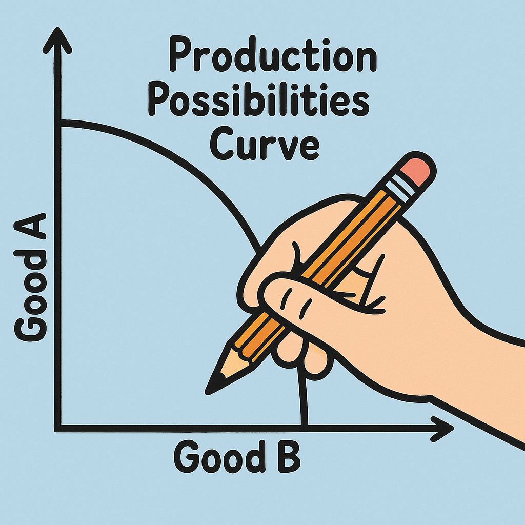
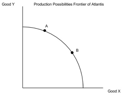
Plotting Potential Production: Hands on with PPC
Students create a combination of posters or bookmarks and then use their production numbers to graph a Production Possibilities Curve.
Key Concepts: AP Microeconomics, Firms and Production, Opportunity Cost…